The pygfx guide

Installation

To install use pip:

pip install -U pygfx

or install the bleeding edge from Github:

pip install -U https://github.com/pygfx/pygfx/archive/main.zip

What is pygfx?

Pygfx is a render engine. It renders objects that are organized in a scene, and provides a way to define what the appearance of these objects should be. For the actual rendering, multiple render backends are available, but the main one is based on WGPU.

The WGPU library provides the low level API to communicate with the hardware. WGPU is itself based on Vulkan, Metal and DX12.

How to use pygfx?

Before jumping into the details, here is a minimal example of how to use the library:

import pygfx as gfx

cube = gfx.Mesh(
    gfx.box_geometry(200, 200, 200),
    gfx.MeshPhongMaterial(color="#336699"),
)

if __name__ == "__main__":
    gfx.show(cube)

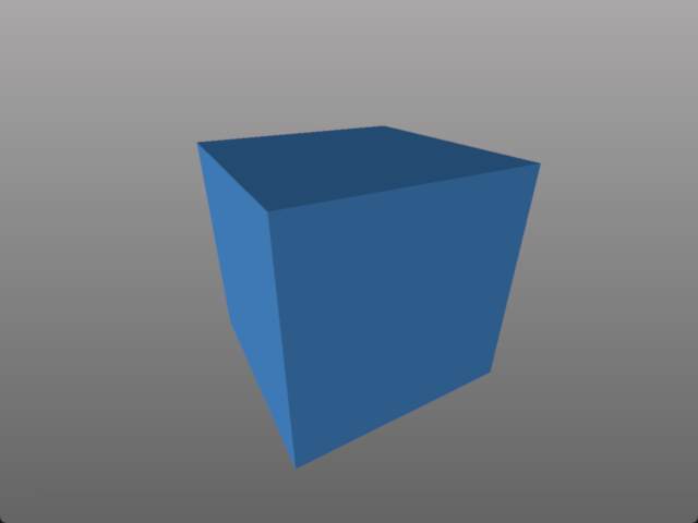
And with that we rendered our first scene using wgpu! Simple, right? At the same time, this is just scratching the surface of what we can do with pygfx and next up we will have a look at the three main building blocks involved in creating more complex rendering setups: (1) Scenes, (2) Canvases, and (3) Renderers.

Scenes

Starting off with the most important building bock, a Scene is the world or scenario to render. It has at least three components: an object with some visual properties, a Light source, and a Camera to view the scene. Once we defined those three things, we can position them within our scene and render it.

Let’s look at an example of how this works and recreate the above example. We begin by defining an empty Scene:

import pygfx as gfx

scene = gfx.Scene()

Right now this scene is very desolate. There is no light, no objects, and nothing that can look at those objects. Let’s change this by adding some light and creating a camera:

# and god said ...
scene.add(gfx.AmbientLight())
scene.add(gfx.DirectionalLight())

camera = gfx.PerspectiveCamera(70, 16 / 9)
camera.local.z = 400

Now there is light and a camera to perceive the light. To complete the setup we also need to add an object to look at:

geometry = gfx.box_geometry(200, 200, 200)
material = gfx.MeshPhongMaterial(color="#336699")
cube = gfx.Mesh(geometry, material)
scene.add(cube)

Objects are slightly more complicated than lights or cameras. They have a geometry, which controls an object’s form, and a material, which controls an object’s appearance (color, reflectiveness, etc). From here, we can hand our result to gfx.show and visualize it. This time, however, we are passing a Scene instead of an Object, so the result will look a little different:

gfx.show(scene)

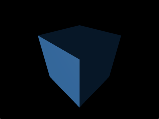
This happens because a complete Scene can be rendered as-is, whereas an Object can not. As such, gfx.show will, when given an Object, create a new scene for us, add the missing lights, a camera, and a background (for visual appeal), place the object into the scene and then render the result. When given a Scene, on the other hand, it will use the input as-is, allowing you to see exactly what you’ve created and potentially spot any problems.

Canvases

The second main building block is the Canvas. A Canvas provides the surface onto which the scene should be rendered, and to use it we directly import it from wgpu-py (on top of which pygfx is built). Wgpu-py has several canvases that we can choose from, but for starters the most important one is auto, which automatically selects an appropriate backend to create a window on your screen:

import pygfx as gfx
from wgpu.gui.auto import WgpuCanvas

canvas = WgpuCanvas(size=(200, 200), title="A cube!")
cube = gfx.Mesh(
    gfx.box_geometry(200, 200, 200),
    gfx.MeshPhongMaterial(color="#336699"),
)

if __name__ == "__main__":
    gfx.show(cube, canvas=canvas)

Like before, gfx.show will automatically create a canvas if we don’t provide one explicitly. This works fine for quick visualizations where the render can appear as a standalone window. However, if we want to have more fine-graned control over the target, e.g., because we want to change the window size or title, we need specify the canvas explicitly. Another common use-case for an explicit canvas is because we are creating a larger GUI and we want the render to only appear in a subwidget of the full window.

Renderers

The third and final main building block is a Renderer. A Renderer is like an artist that brings all of the above together. It looks at the Scene through a Camera and draws what it sees onto the surface provided by the Canvas. Like any good artist, a Renderer is never seen without its Canvas, so to create a Renderer we also need to create a Canvas:

import pygfx as gfx
from wgpu.gui.auto import WgpuCanvas

canvas = WgpuCanvas()
renderer = gfx.renderers.WgpuRenderer(canvas)

cube = gfx.Mesh(
    gfx.box_geometry(200, 200, 200),
    gfx.MeshPhongMaterial(color="#336699"),
)

if __name__ == "__main__":
    gfx.show(cube, renderer=renderer)

The output is the same as without the explicit reference because gfx.show will, as you may expect at this point, create a renderer if we don’t provide it. For many applications this is perfectly fine; however, if we want to tackle more advanced problems (e.g., control the exact process on how objects appear to overlay each other) we may need to create it explicitly. For starters, it is enough to know that it exists and what it does, so that we can come back to it later when it becomes relevant.

Animations

Static renders are nice, but you know what is better? Animations! As mentioned in the section on Canvases, this is done via a backend’s event loop which allows you to specify callbacks that get executed periodically. For convenience, gfx.show exposes two callbacks that will be executed before a new render is made (before_render) and afterward (after_render). To animate a scene, simply pass a callback to this function (here animate) and use it to modify the scene as desired:

import pygfx as gfx
import pylinalg as la

cube = gfx.Mesh(
    gfx.box_geometry(200, 200, 200),
    gfx.MeshPhongMaterial(color="#336699"),
)

rot = la.quat_from_euler((0, 0.01), order="XY")

def animate():
    cube.local.rotation = la.quat_mul(rot, cube.local.rotation)

if __name__ == "__main__":
    gfx.show(cube, before_render=animate)

World objects

We’ve briefly mentioned world objects, materials, and geometry. But how do these relate?

A world object represents an object in the world. It has a transform, by which the object can be positioned (translated, rotated, and scaled), and has a visibility property. These properties apply to the object itself as well as its children (and their children, etc.).

All objects that have an appearance in the scene are world objects. But there are also helper objects, lights, and cameras. These are all world objects.

Geometry

Most world objects have a geometry. This geometry object contains the data that defines (the shape of) the object, such as positions, plus data associated with these positions (normals, texcoords, colors, etc.). Multiple world objects may share a geometry.

Materials

All world objects that have an appearance, have a material that defines that appearance. (Objects that do not have an appearance are for example groups or cameras.) For each type of object there are typically a few different material classes, e.g. for meshes you have a MeshBasicMaterial that is not affected by lights, a MeshPhongMaterial that applies the Phong light model, and the MeshStandardMaterial that implements a physically-based light model. Materials also have properties to tune things like color, line thickness, colormap, etc. Multiple world objects may share the same material object, so their appearance can be changed simultaneously.

Cameras and controllers

We’ve already been using cameras, but let’s look at them a bit closer!

Perspective camera

There are two main cameras of interest. The first is the PerspectiveCamera, which is a generic camera intended for 3D content. You can instantiate one like this:

camera = gfx.PerspectiveCamera(50, 4/3)

The first argument is the fov (field of view) in degrees. This is a value between 0 and 179, with typical values < 100. The second argument is the aspect ratio. A window on screen is usually a rectangle with 4/3 or 16/9 aspect. The aspect can be set so the contents better fit the window. When the fov is zero, the camera operates in orthographic mode.

Orthographic camera

The second camera of interest is the OrthographicCamera. Technically it’s a perspective camera with the fov fixed to zero. It is also instantiated differently:

camera = gfx.OrthographicCamera(500, 400, maintain_aspect=False)

The first two arguments are the width and height, which are typically used to initialize an orthographic camera. This implicitly sets the aspect (which is the width divided by the height). The maintain_aspect argument can be set to False if the dimensions do not represent a physical dimension, e.g. for plotting data. The contents of the view are then stretched to fill the window.

Orienting cameras

Camera’s can be oriented manually by setting their position, and then set their rotation to have them look in the correct direction, e.g. using .look_at(). In this case you should probably set the width in addition to fov and aspect.

# Manual orientation
camera = gfx.PerspectiveCamera(50, 4/3, width=100)
camera.local.position = (30, 40, 50)
camera.look_at((0, 0, 0))

However, we strongly recommend using one of the show methods, since these also set the width and height. Therefore they better prepare the camera for controllers, and the near and far clip planes are automatically set.

# Create a camera, in either way
camera = gfx.PerspectiveCamera(50, 4/3)
camera = gfx.OrthographicCamera()

# Convenient orientation: similar to look_at
camera.local.position = (30, 40, 50)
camera.show_pos((0, 0, 0))

# Convenient orientation: show an object
camera.show_object(target, view_dir=(-1, -1, -1))

# Convenient orientation: show a rectangle
camera.show_rect(0, 1000, -5, 5, view_dir=(0, 0, -1))

The .show_pos() method is the convenient alternative for look_at. Even easier is using .show_object(), which allows you to specify an object (e.g. the scene) and optionally a direction. The camera is then positioned and rotated to look at the scene from the given direction. A similar method, geared towards 2D data is .show_rect() in which you specify a rectangle instead of an object.

The near and far clip planes

Camera’s cannot see infinitely far; they have a near and far clip plane. Only the space between these planes can be seen. To get a bit more technical, this space is mapped to a value between 0 and 1 (NDC coordinates), and this is converted to a depth value. Since the number of bits for depth values is limited, it’s important for the near and far clip planes to have reasonable values, otherwise you may observe “z fighting”, or objects may simply not be visible.

If you use the recommended show methods mentioned above, the near and far plane are positioned about 1000 units apart, scaled with the mean of the camera’s width and height. If needed, the clip planes can be specified explicitly using the depth_range property.

Controlling the camera

A controller allows you to interact with the camera using the mouse. You simply pass the camera to control when you instantiate it, and then make it listen to events by connecting it to the renderer or a viewport.

controller = gfx.OrbitController(camera)
controller.add_default_event_handlers(renderer)

There are currently two controllers: the PanZoomController is for 2D content or in-plane visualization, and the OrbitController is for 3D content. All controllers work with both perspective and orthographic cameras.

Updating transforms

WorldObjects declare two reference frames that we can use to maneuver them around: local and world. local allows us to position an object relative to its parent and world allows us to position objects relative to the world’s inertial frame.

Note

Both local and world declare the same properties, meaning that we can express any of the below properties in either frame.

cube = gfx.Mesh(
    gfx.box_geometry(10, 10, 10),
    gfx.MeshPhongMaterial(color="#808080"),
)

cube.world.position = (1, 2, 3)
cube.world.rotation = la.quat_from_euler(
    (np.pi/2, np.pi/2), order="YX"
)
cube.world.scale = (2, 4, 6)
cube.world.scale = 3  # uniform scale

# setting components only
cube.local.x = 1
cube.local.y = 10
cube.local.z = 100

cube.local.scale_x = 2
cube.local.scale_y = 4
cube.local.scale_z = 6

Warning

While in-place updating of full properties is supported, in-place updating of slices will have no effect. This is due to limitations of the python programming language and our desire to have the properties return pure numpy arrays. In code, this means

cube.local.position += (0, 0, 3)  # ok
cube.local.z += 3  # ok
cube.local.position[2] += 3  # FAIL: this will have no effect.
cube.local.position[2] = 3  # FAIL: this will have no effect.

Beyond setting components, we can also set the full matrix directly:

cube.world.matrix = la.mat_from_translation((1, 2, 3))

and we can - of course - read each property. To make a full example, we can create a small simulation of a falling and rotating cube.

import numpy as np
import pygfx as gfx
import pylinalg as la

companion_cube = gfx.Mesh(
    gfx.box_geometry(1, 1, 1),
    gfx.MeshPhongMaterial(color="#808080"),
)
companion_cube.world.position = (0, 100, 0)

# add an IMU sensor to the corner of the cube (IMUs measure acceleration)
imu_sensor = gfx.WorldObject()
companion_cube.add(imu_sensor)
imu_sensor.local.position = (0.5, 0.5, 0.5)
imu_mass = 0.005  # kg

# obligatory small rotation
rot = la.quat_from_euler((0.01, 0.05), order="XY")
axis, angle = la.quat_to_axis_angle(rot)

# simulate falling cube
gravity = -9.81 * companion_cube.world.reference_up
velocity = np.zeros(3)
update_frequency = 1 / 50  #  Hz
for _ in range(200):
    # the cube is falling
    velocity = velocity + update_frequency * gravity
    companion_cube.world.position += update_frequency * velocity

    # and spinning around.
    companion_cube.local.rotation = la.quat_mul(
        rot, companion_cube.local.rotation
    )

    # The sensor has some velocity relative to the companion cube as it rotates
    # around the latter
    angular_moment = angle / update_frequency
    velocity_rotation = np.cross(angular_moment * axis, imu_sensor.local.position)

    # and is thus experiencing both gravity and centripetal forces
    local_gravity = -9.81 * imu_sensor.local.reference_up
    local_centripetal = np.cross(angular_moment * axis, velocity_rotation)

    # The IMU thus measures the composite of the above accelerations
    observed_acceleration = local_gravity + local_centripetal

    total_g = np.linalg.norm(observed_acceleration) / 9.81
    print(f"Feels like: {total_g:.3} g")

Colors

Colors in Pygfx can be specified in various ways, e.g.:

material.color = "red"
material.color = "#ff0000"
material.color = 1, 0, 0

Most colors in Pygfx contain four components (including alpha), but can be specified with 1-4 components:

• a scalar: a grayscale intensity (alpha 1).

• two values: grayscale intensity plus alpha.

• three values: red, green, and blue (i.e. rgb).

• four values: rgb and alpha (i.e. rgba).

Colors for the Mesh, Point, and Line

These objects can be made a uniform color using material.color. More sophisticated coloring is possible using colormapping and per-vertex colors.

For Colormapping, the geometry must have a .texcoords attribute that specifies the per-vertex texture coordinates, and the material should have a .map attribute that is a texture in which the final color will be looked up. The texture can be 1D, 2D or 3D, and the number of columns in the geometry.texcoords should match. This allows for a wide variety of visualizations.

Per-vertex or per-face colors can be specified as geometry.colors. They must be enabled by setting material.color_mode to “vertex” or “face”. The colors specified in material.map and in geometry.colors can have 1-4 values.

Colors in Image and Volume

The values of the Image and Volume can be either directly interpreted as a color or can be mapped through a colormap set at material.map. If a colormap is used, it’s dimension should match the number of channels in the data. Again, both direct and colormapped colors can be 1-4 values.

Colorspaces

All colors in pygfx are interpreted as sRGB by default. This is the same how webbrowsers interpret colors. Internally, all calculations are performed in the physical colorspace (sometimes called Linear sRGB) so that these calculations are physically correct.

If you create a texture with color data that is already in physical/linear colorspace, you can set the Texture’s colorspace argument to “physical”.

Similarly you can use Color.from_physical() to convert a physical color to sRGB.

Using Pygfx in Jupyter

You can use Pygfx in the Jupyter notebook and Jupyter lab. To do so, use the Jupyter canvas provided by WGPU, and use that canvas as the cell output.

from wgpu.gui.jupyter import WgpuCanvas

canvas = WgpuCanvas()
renderer = gfx.renderers.WgpuRenderer(canvas)

...

canvas  # cell output

Also see the Pygfx examples here.